课程介绍

台湾交通大学吴庆堂老师随机分析，课程视频：金融随机分析.

参考网站：國立交通大學開放式課程 (NCTU OCW).

参考资料：北京大学数学科学学院金融数学系《金融中的随机数学》1班的讲义.

参考讲义： Selected Topics in Learning, Prediction and Optimization

期望与积分

Definition 1.21. The function $$ \mathbb{I}_A(\omega)= \begin{cases}0, & \text { if } \omega \notin A \\ 1, & \text { if } \omega \in A\end{cases} $$ is called the indicator function of $A$.

Remark 1.22. The indicator function $\mathbb{I}_A$ is a random variable if and only if $A \in \mathcal{F}$.

严格的定义积分，需要从最简单的情况开始，即形状类似为阶跃函数的非负随机变量，然后减少阶跃平台的长度（取极限），得到简单情况的积分，再构造 $X = X^{+}-X^{-}$,使得 $X^{+},X^{-}$ 都非负的方式满足一般的r.v.，如此便可以严格的定义积分，这里直接给出定义。

Definition 1.26. Consider a general random variable $X$. Then we can write $X$ as $$ X=X^{+}-X^{-} $$ where $X^{+}=X \vee 0, X^{-}=(-X) \vee 0$.
(1) Unless both of $\mathbb{E}\left[X^{+}\right]$and $\mathbb{E}\left[X^{-}\right]$are $+\infty$, we define
$$ \mathbb{E}[X]=\mathbb{E}\left[X^{+}\right]-\mathbb{E}\left[X^{-}\right] $$ (2) If $\mathbb{E}|X|=\mathbb{E}\left[X^{+}\right]+\mathbb{E}\left[X^{-}\right]<\infty, X$ has a finite expectation. We denote by $$ \mathbb{E}[X]=\int_{\Omega} X d \mathbb{P}=\int_{\Omega} X(\omega) \mathbb{P}(d \omega) $$ (3) For $A \in \mathcal{F}$, define $$ \int_A X d \mathbb{P}=\mathbb{E}\left[X \mathbb{I}_A\right] $$ which is called the integral of $X$ with respect to $\mathbb{P}$ over $A$.
(4) $X$ is integrable with respect to $\mathbb{P}$ over $A$ if the integral exists and is finite.

这种积分为 Lebesgue integral，是一种带测度的积分，与黎曼积分的定义方式不同：黎曼积分是在定义域上进行切分，而Lebesgue integral是对值域进行切分，并且其横坐标是带有测度的，对于随机变量来说，横坐标的测度和为 $1$.可以将 Lebesgue integral理解为求一种面积（或者高度，因为横坐标全体的测度为1）.

Lebesgue integral和黎曼积分的性质有很多相似之处，这里对一些符合直觉的性质就不一一列举，下面给出一个Lebesgue integral独有的性质：

Proposition 1.29.(Absolute Integrability) $$ \int_A X d \mathbb{P}<\infty \quad \Longleftrightarrow \quad \int_A|X| d \mathbb{P}<\infty . $$

条件期望和条件概率

初等概率论中没有条件期望是随机变量的概念，所定义的条件概率也仅仅是数值，只可以处理对于某一特定条件下的概率，但是条件期望应该是对所以可能发生的事件作为given来说的，所以我们有必要更严谨的处理这一点。

吴庆堂老师关于条件期望的定义讲的很棒，本人看过一些高等概率论的讲义，均没有吴庆堂老师老师的定义方式更加循循善诱，吴庆堂老师先从普通的集合条件概率开始，然后构造 $\Omega$ 的 decomposition 作为条件,再构造由离散型r.v.诱导的decomposition，最后根据直觉定义以 $\sigma-$代数作为条件的条件期望，再诱导出条件概率，十分精彩，现在我们来也拙略的模仿这种形式，依照直觉导出条件期望这个在初等概率论中触不可及的名词。

基于集合的条件概率是容易定义的，基于随机变量的确定取值求取条件概率也是初等概率论中就提到的东西，我们这里从$\Omega$ 的 decomposition开始，进行描述。

Consider a probability space $(\Omega, \mathcal{F}, \mathbb{P})$. Let $\mathcal{D}=\left\{D_1, D_2, \ldots, D_n\right\}$ satisfy
(1) $\mathcal{D}$ is a decomposition of $\Omega$, i.e., $$ D_1 \cup D_2 \cup \cdots \cup D_n=\Omega, \quad D_i \cap D_j=\emptyset \quad \text { for } i \neq j ; $$ (2) $D_i \in \mathcal{F}$ for all $i$;
(3) $\mathbb{P}\left(D_i\right)>0$ for all $i$.
Therefore, for $A \in \mathcal{F}$, the conditional probability $\mathbb{P}\left(A \mid D_i\right)$ is well-defined for all $i$.

Definition 2.12. The conditional probability of a set $A \in \mathcal{F}$ with respect to the decomposition $\mathcal{D}$ is defined by $$ \mathbb{P}(A \mid \mathcal{D})=\sum_{i=1}^n \mathbb{P}\left(A \mid D_i\right) \mathbb{I}_{D_i} $$ Remark. $\mathbb{P}(A \mid \mathcal{D})$ is a random variable and $$ \mathbb{P}(A \mid \mathcal{D})=\sum_{i=1}^n \mathbb{P}\left(A \mid D_i\right) \mathbb{I}_{D_i} $$ This implies that if $\omega \in D_i, \mathbb{P}(A \mid \mathcal{D})(\omega)=\mathbb{P}\left(A \mid D_i\right)$.

这种方式就是把整个 $\Omega$ 划分为互不相交的 $D_i$,不同的 $D_i$ 上条件概率有不同的取值，这不正像一个离散型的随机变量呢，所以用离散型随机变量诱导划分 $\Omega$ 是很自然的行为：

Let $$ Y=\sum_{i=1}^n y_i \mathbb{I}_{D_i} $$ where $y_1, y_2, \ldots, y_n$ are distinct constants, and $\left\{D_1, D_2, \ldots, D_n\right\}$ is a decomposition of $\Omega$ with $\mathbb{P}\left(D_i\right)>0$ for all $i$. Then $$ D_i=\left\{Y=y_i\right\} $$

Definition 2.15.
(1) $\mathcal{D}_Y=\left\{D_1, D_2, \ldots, D_n\right\}$ is called the decomposition induced by $Y$.
(2) $\mathbb{P}(A \mid Y):=\mathbb{P}\left(A \mid \mathcal{D}_Y\right)$ is called the conditional probability of $A$ with respect to the random variable $Y$. Moreover, we denote by $\mathbb{P}\left(A \mid Y=y_i\right)$ the conditional probability $\mathbb{P}\left(A \mid D_i\right)$.

实际上，该离散型随机变量的功能就是划分样本空间，所以事件 $A$ 在不同的划分后样本空间上自然会有不同的取值，这种定义方式可以代替上述简单的划分，所以，这两种定义本质上是同一种定义，它们诱导出的条件期望非常直观：

Definition 2.17. The conditional expectation of $X$ with respect to a decomposition $\mathcal{D}=\left\{D_1, D_2, \ldots, D_n\right\}$ is defined by $$ \mathbb{E}[X \mid \mathcal{D}]=\sum_{i=1}^m x_i \mathbb{P}\left(A_i \mid \mathcal{D}\right) $$ Remark. 一种对该公式的理解： $$ \begin{aligned} \mathbb{E}[X \mid \mathcal{D}] & =\sum_{i=1}^m x_i \mathbb{P}\left(A_i \mid \mathcal{D}\right)=\sum_{i=1} x_i \sum_{j=1}^n \mathbb{P}\left(A_i \mid D_j\right) \mathbb{I}_{D_j} \\ & =\sum_{j=1}^n \mathbb{E}\left[\sum_{i=1}^m x_i \mathbb{I}_{A_i} \mid D_j\right] \mathbb{I}_{D_j}=\sum_{j=1}^n \mathbb{E}\left[X \mid D_j\right] \mathbb{I}_{D_j} . \end{aligned} $$ 其中用到了一种性质：$\mathbb{E}\left[\mathbb{I}_A \mid \mathcal{D}\right]=\mathbb{P}(A \mid \mathcal{D})$，并假设 $X$ 就是上面公式中的随机变量；通过该公式可以明了的看出条件期望是随机变量，在不同的 $D_i$ 下有不同的值。

这里给出一个例子强化我们的直觉：

Example 2.20. Let $(\Omega, \mathcal{F}, \mathbb{P})=\left([0,1], \mathcal{B}_1, m\right), \mathcal{D}=\{[0,1 / 2),[1 / 2,1]\}=\left\{D_1, D_2\right\}$ and $$ X=\mathbb{I}_{[0,1.3]}+2 \mathbb{I}_{(1 / 3,2 / 3)}+3 \mathbb{I}_{[2 / 3,1]} . $$ we have $$ \mathbb{E}[X \mid \mathcal{D}]=\mathbb{E}\left[X \mid D_1\right] \mathbb{I}_{D_1}+\mathbb{E}\left[X \mid D_2\right] \mathbb{I}_{D_2} $$ Moreover, $$ \begin{aligned} \mathbb{E}\left[X \mid D_1\right] & =\mathbb{P}\left([0,1 / 3] \mid D_1\right)+2 \mathbb{P}\left((1 / 3,2 / 3) \mid D_1\right)+3 \mathbb{P}\left([2 / 3,1] \mid D_1\right) \\ & =\frac{1 / 3}{1 / 2}+2 \cdot \frac{1 / 6}{1 / 2}=\frac{4}{3} \end{aligned} $$ $$ \begin{aligned} \mathbb{E}\left[X \mid D_2\right] & =\mathbb{P}\left([0,1 / 3] \mid D_2\right)+2 \mathbb{P}\left((1 / 3,2 / 3) \mid D_2\right)+3 \mathbb{P}\left([2 / 3,1] \mid D_2\right) \\ & =2 \cdot \frac{1 / 6}{1 / 2}+3 \cdot \frac{1 / 3}{1 / 2}=\frac{8}{3} \end{aligned} $$ Thus, $$ \mathbb{E}[X \mid \mathcal{D}]=\frac{4}{3} \mathbb{I}_{D_1}+\frac{8}{3} \mathbb{I}_{D_2} $$ 该图像告诉我们一点：条件期望在给定区间 $($D_1,D_2$)$ 下的面积和原有面积一致，高度是其带比例平均。

有了这些直觉，我们再给出条件期望的定义：

Definition 2.21. The conditional expectation of $X$ with respect to $\mathcal{G}$ is a nonnegative random variable denoted by $\mathbb{E}[X \mid \mathcal{G}]$ or $\mathbb{E}[X \mid \mathcal{G}](\omega)$, such that
(i) $\mathbb{E}[X \mid \mathcal{G}]$ is $\mathcal{G}$-measurable $\iff\{\mathbb{E}[X \mid \mathcal{G}] \leq C\} \in \mathcal{G}$ for all $C$.
(ii) For all $A \in \mathcal{G}$, $$ \int_A \mathbb{E}[X \mid \mathcal{G}] d \mathbb{P}=\int_A X d \mathbb{P} $$ Remark. 第一个条件说明给定 $\mathcal{G}$ 可以求得条件期望；第二个条件说明条件期望的平均高度（或者面积）和原来的随机变量的高度（或者面积）一致。

我们不加讨论的说明这一点：在排除零测集的意义下，条件期望存在且唯一。这说明条件期望是Well-define的，我们现在来思考这样的条件期望是否符合我们的“直觉”。

定义的条件（1）是毋庸置疑的，当我们给定了划分的具体区域，是可以求得条件期望的具体值的，这句话其实隐含了一件事情：$\sigma-$域可以看作对 $\Omega$ 的划分！为什么对于一般的随机变量条件期望如此难定义，正是因为对样本空间难以划分，given的条件可以将 $\Omega$ 划分为极其复杂的程度，所以我们需要更强力的 $\sigma-$域对这种划分进行描述，按照以前的情况，即 $\mathcal{G} = \sigma (\left\{D_1,D_2,\cdots,D_n\right\}) $.

从另外一个角度来理解，$\sigma-$域表示一种information，在这里，就是指随机变量在given的information下的期望值，不同的information自然会有不同的期望值。

我们现在给出一个例子，来理解这个定义：

Example 2.23. (1) Consider a probability space $\left([0,1], \mathcal{B}_1, m\right)$. Let $X$ be uniformly distributed on $[0,1]$ and let $$ \mathcal{G}=\sigma\left(\left\{0 \leq X<\frac{1}{2}\right\},\left\{\frac{1}{2} \leq X \leq 1\right\}\right) $$

Sol:Using the definition of condition expectation: By Definition 2.21 (i), we see that $$ \mathbb{E}[X \mid \mathcal{G}]=c_1 \mathbb{I}_{\left\{0 \leq X<\frac{1}{2}\right\}}+c_2 \mathbb{I}_{\left\{\frac{1}{2} \leq X \leq 1\right\}} $$ For $A=\left\{0 \leq X<\frac{1}{2}\right\}$,

By Definition 2.21 (ii), we see that $$ \frac{c_1}{2}=\frac{1}{8} $$ Hence, $c_1=1 / 4$. Similarly, we can get $c_2=3 / 4$. Thus, $$ \mathbb{E}[X \mid \mathcal{G}]=\frac{1}{4} \mathbb{I}_{\left\{0 \leq X<\frac{1}{2}\right\}}+\frac{3}{4} \mathbb{I}_{\left\{\frac{1}{2} \leq X \leq 1\right\}} $$

可见，由于 $\sigma-$域的划分，每个划分区域有不同的条件期望，由于 $\sigma-$域可以描述复杂的划分，上述定义也可以应对更复杂的情况，而定义中的条件（2），则是可以帮助我们求得条件概率具体值的必要条件：面积一致。

上述定义的是非负的情况，很简单的可以推广到一般的条件期望：

Definition 2.24. The conditional expectation $\mathbb{E}[X \mid \mathcal{G}]$, or $\mathbb{E}[X \mid \mathcal{G}](\omega)$, of any random variable with respect to the $\sigma$-algebra $\mathcal{G}$, is defined by $$ \mathbb{E}[X \mid \mathcal{G}]=\mathbb{E}\left[X^{+} \mid \mathcal{G}\right]-\mathbb{E}\left[X^{-} \mid \mathcal{G}\right] $$ if $\min \left\{\mathbb{E}\left[X^{+} \mid \mathcal{G}\right], \mathbb{E}\left[X^{-} \mid \mathcal{G}\right]\right\}<\infty \mathbb{P}$-a.s. On the set of sample points for which $\mathbb{E}\left[X^{+} \mid \mathcal{G}\right]=$ $\mathbb{E}\left[X^{-} \mid \mathcal{G}\right]=\infty, \mathbb{E}\left[X^{+} \mid \mathcal{G}\right]-\mathbb{E}\left[X^{-} \mid \mathcal{G}\right]$ is given by an arbitrary value.

Definition 2.25. Let $B \in \mathcal{F}$. The conditional probability of $B$ with respect to $\mathcal{G}$ is defined by $$ \mathbb{P}(B \mid \mathcal{G})=\mathbb{E}\left[\mathbb{I}_B \mid \mathcal{G}\right] $$

下面给出条件期望的性质，这些性质在后面的分析中非常有用：

Proposition 2.26.
(1) If $X \equiv C \mathbb{P}$-a.s., then $\mathbb{E}[X \mid \mathcal{G}]=C \mathbb{P}$-a.s.
(2) If $X \leq Y \mathbb{P}$-a.s., then $\mathbb{E}[X \mid \mathcal{G}] \leq \mathbb{E}[Y \mid \mathcal{G}] \mathbb{P}$-a.s.
(3) $|\mathbb{E}[X \mid \mathcal{G}]| \leq \mathbb{E}[|X| \mid \mathcal{G}] \mathbb{P}$-a.s.
(4) For constants $a, b$ with $a \mathbb{E}[X]+b \mathbb{E}[Y]<\infty$, then $$ \mathbb{E}[a X+b Y]=a \mathbb{E}[X]+b \mathbb{E}[Y] $$ (5) Consider the trivial $\sigma$-algebra $\mathcal{F}^{*}=\{\emptyset, \Omega\}$. Then $$ \mathbb{E}\left[X \mid \mathcal{F}^{*}\right]=\mathbb{E}[X], \quad \mathbb{P} \text { - a.s. } $$ (6) If $X$ is $\mathcal{G}$-measurable, then $\mathbb{E}[X \mid \mathcal{G}]=X$.
(7) $\mathbb{E}[\mathbb{E}[X \mid \mathcal{G}]]=\mathbb{E}[X]$.
(8) (Tower property) If $\mathcal{G}_1 \subset \mathcal{G}_2$, then $$ \mathbb{E}\left[\mathbb{E}\left[X \mid \mathcal{G}_1\right] \mid \mathcal{G}_2\right]=\mathbb{E}\left[X \mid \mathcal{G}_1\right]=\mathbb{E}\left[\mathbb{E}\left[X \mid \mathcal{G}_2\right] \mid \mathcal{G}_1\right] $$ (9) Let $Y$ be $\mathcal{G}$-measurable with $\mathbb{E}|X|<\infty, \mathbb{E}|X Y|<\infty$. Then $$ \mathbb{E}[X Y \mid \mathcal{G}]=Y \mathbb{E}[X \mid \mathcal{G}], \quad \mathbb{P} \text { - a.s. } $$

Remark 2.28. Denote $$ \sigma(Y)=\left\{\{\omega: Y(\omega) \in B\}: B \in \mathcal{B}^1\right\}=\sigma(\{Y \leq r\}): r \in \mathbb{R} . $$

Proposition 2.29. If $Y$(means $\sigma(Y)$) and a $ \sigma$-algebra $\mathcal{G}$ are independent , $$ \mathbb{E}[Y \mid \mathcal{G}]=\mathbb{E}[Y] $$

离散鞅

鞅

Definition 2.30(信息流). (1) A sequence of $\sigma$-algebra $\left(\mathcal{F}_n\right)_{n \geq 1}$ is called a filtration if $\mathcal{F}_n \subseteq$ $\mathcal{F}_{n+1}$ for all $n \geq 1$.
(2) A probability space $(\Omega, \mathcal{F}, \mathbb{P})$ with filtration $\mathbb{F}=\left(\mathcal{F}_n\right)$ is called a filtered probability space, and is denoted by $(\Omega, \mathcal{F}, \mathbb{F}, \mathbb{P})$ or $\left(\Omega, \mathcal{F},\left(\mathcal{F}_n\right), \mathbb{P}\right)$.

Definition 2．32（鞅）. Let $\left(X_n\right)_{n \geq 1}$ be a sequence of random variables and $\left(\mathcal{F}_n\right)_{n \geq 1}$ is a filtration．We say $\left(X_n, \mathcal{F}_n\right)$ is a martingale（平赌，鞅 or say $\left(X_n\right)$ is a martingale with respect to $\left(\mathcal{F}_n\right),\left(X_n\right)$ is an $\left(\mathcal{F}_n\right)$－martingale）if
（a）（适应性）$X_n \in \mathcal{F}_n$ for all $n$ ，i．e．，$\left(X_n\right)$ is $\left(\mathcal{F}_n\right)$－adapted,measurable；
（b） （可积）$\mathbb{E}\left|X_n\right|<\infty$ for all $n$ ；
（c）(鞅性)$X_n=\mathbb{E}\left(X_{n+1} \mid \mathcal{F}_n\right), \mathbb{P}$－a．s．for all $n$ ．
Remark 2.33. The condition (c) in Definition 2.32 is equivalent to
$\left(c^{\prime}\right) X_n=\mathbb{E}\left(X_m \mid \mathcal{F}_n\right)$ for all $m>n$.
$\left(\mathrm{c}^{\prime \prime}\right) \int_A X_n d \mathbb{P}=\int_A X_m d \mathbb{P}$ for all $A \in \mathcal{F}_n$ and for all $m>n$.

鞅和其信息流以及测度息息相关，我们可以通过一些测度变换的手段，让鞅变成非鞅，也可以让非鞅变成鞅。

Definition 2．37．保持鞅定义的第一第二条，有：
（1）$\left(X_n\right)$ is an $\left(\mathcal{F}_n\right)$－submartingale（优赌，下鞅）if $X_n \leq \mathbb{E}\left(X_{n+1} \mid \mathcal{F}_n\right)$ for all $n P$－a．s．
（2）$\left(X_n\right)$ is an $\left(\mathcal{F}_n\right)$－supermartingale（劣赌，上鞅）if $X_n \geq \mathbb{E}\left(X_{n+1} \mid \mathcal{F}_n\right)$ for all $n P$－a．s．
Remark. 鞅既是上鞅也是下鞅。

Theorem 2.39(构造下鞅). Let $\left(X_n, \mathcal{F}_n\right)$ be a submartingale and let $\varphi$ be an increasing convex function defined on $\mathbb{R}$. If $\varphi\left(X_n\right)$ is integrable for all $n$, then $\left(\varphi\left(X_n\right)\right)$ is a submartingale w.r.t. $\mathcal{F}_n$.

鞅变换和Doob分解

Definition 2.45（可预测过程）. If $M_n \in \mathcal{F}_{n-1}$ for all $n$, we say that the stochastic process $\left(M_n\right)$ is an $\left(\mathcal{F}_n\right)$-predictable process.

Definition 2.46(鞅变换).
(1) Let $\left(X_n, \mathcal{F}_n\right)$ be a stochastic process and let $M=\left(M_n, \mathcal{F}_{n-1}\right)$
be a predictable process, then the stochastic process $$ (M \cdot X)_n=M_0 X_0+\sum_{i=1}^n M_i\left(X_i-X_{i-1}\right) $$ is called the transform of $X$ by $M$.
(2) If, in addition, $X$ is a martingale, we say that $M \cdot X$ is a martingale transform.
Remark. 若 $M_n$ 可积分，则上述变换是鞅变换。

Definition 2.48（增长过程）. A sequence of random variables $\left(Z_n\right)$ is called an increasing process if
(1) $Z_1=0$ and $Z_n \leq Z_{n+1}$ for all $n \geq 1$.
(2) $\mathbb{E}\left(Z_n\right)<\infty$ for all $n$.

Theorem 2.50 (Doob decomposition). Any submartingale $\left(X_n, \mathcal{F}_n\right)$ can be written as $$ X_n=Y_n+Z_n, $$ where $\left(Y_n, \mathcal{F}_n\right)$ is a martingale and $\left(Z_n\right)$ is an increasing predictable process.
Remark. 下鞅可以分解为增长过程和鞅，这也是符合直觉的定理。值得注意的是，这种分解是唯一的。

停时

Consider a probability space $(\Omega, \mathcal{F}, \mathbb{P})$ with filtration $\mathbb{F}=\left(\mathcal{F}t\right){t=0,1,2, \ldots, T}$.

Definition 5.1(停时). A random variable $\tau: \Omega \longrightarrow{0,1,2, \ldots, T} \cup{+\infty}$ is called a stopping time with respect to $\mathbb{F}$ if $$ {\tau=t} \in \mathcal{F}_t $$ for all $t$.
Remark. 可见，停时是一个随机变量，引入停时就是因为我们想描述截止到事件发生时间的信息量，注意，该定义是离散时间的停时，我们在后续章节会定义连续时间的停时。

Definition 5.4（停时生成的$\sigma$代数）. Let $\tau$ be a stopping time, then $$ \mathcal{F}_\tau:=\left\{A \in \mathcal{F}: A \cap\{\tau \leq t\} \in \mathcal{F}_t \text { for all } t \leq T\right\} $$ is called the $\sigma$-algebra of events determined prior to the stopping time $\tau$.
Remark. 具体的例子可以在课程的讲义上找，这里用一种直观的方式说明：该 $\sigma$代数是使得截止到当前停止时间能获得的最细分的 $\sigma$代数，即我们在停时时刻能得到的最大信息量（由我们在条件期望章节的直观：$\sigma$代数就是信息量，就是将空间进行划分，这种定义可以基于现有的观测，将空间分的最细）。

Lemma 5.7（停时诱导的随机变量）. Let $\tau$ be a stopping time, then the random variable $$ X_\tau(\omega):=X_{\tau(\omega)}(\omega) $$ is $\mathcal{F}_\tau$-measurable.

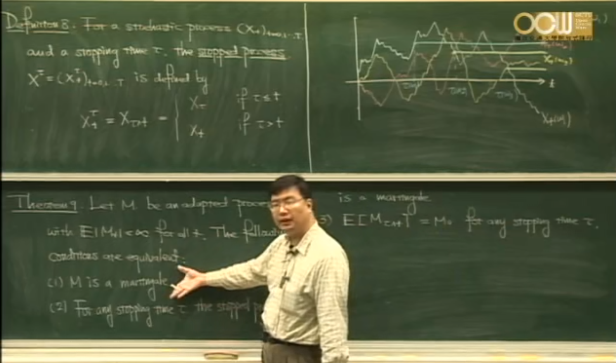
Definition 5.8（停时过程）. For a stochastic process $X=\left(X_t\right)_{0 \leq t \leq T}$ and a stopping time $\tau$, the stopped process $X^\tau=\left(X_t^\tau\right)_{0 \leq t \leq T}$ is defined by $$ X_t^\tau=X_{\tau \wedge t}:= \begin{cases}X_\tau, & \text { if } \tau \leq t \\ X_t, & \text { if } \tau>t\end{cases} $$

Theorem 5.9(停时鞅). Let $M$ be an adapted process with $M_t \in L^1(\mathbb{Q})$ for each $t$. Then the following statements are equivalent.
(1) $M$ is a $\mathbb{Q}$-martingale;
(2) For any stopping time $\tau$, the stopped process $M_{\tau \wedge t}$ is a $\mathbb{Q}$-martingale;
(3) $\mathbb{E}_{\mathbb{Q}}\left[M_{\tau \wedge t}\right]=M_0$ for any stopping time $\tau$.

连续时间随机过程

从离散时间随机过程到连续时间随机过程发生了非常大的跳跃，最主要是因为域流 $\mathcal{F}_t$ 的理解变得困难，我们无法举出一些很好的例子，只能沿用从离散观点带来的直觉。

随机过程

Let $(\Omega, \mathcal{F}, \mathbb{P})$ be a probability space and let $I \subset[0, \infty)$ be an interval．

Definition 7．1（随机过程）． A real－valued stochastic process $X=\left(X_t\right)_{t \in I}$ is a family of random variables $\left(X_t: t \in I\right)$ on $(\Omega, \mathcal{F})$ ． ．

Remark 7.2 (经典解释方法：二元函数).（1）We may regard the stochastic process $X$ as a function of two variables $$ \begin{aligned} X: I \times \Omega & \longrightarrow \mathbb{R} \\ (t, \omega) & \longmapsto X_t(\omega) \end{aligned} $$ （2）For fixed $\omega \in \Omega$ ，then $$ t \longmapsto X_t(\omega) $$ is a function：$I \longrightarrow \mathbb{R}$ ，which is called a path of $X$ ．
（3）For fixed $t \in I$ ，then $$ \omega \longmapsto X_t(\omega) $$ is a function：$\Omega \longrightarrow \mathbb{R}$ ，which is a random variable．

Definition 7．3（usual condition）．（1）A filtration $\mathbb{F}=\left(\mathcal{F}_t\right)_{t \in I}$ is a family of $\sigma$－algebras satisfying $$ \mathcal{F}_s \subseteq \mathcal{F}_t $$ for all $s, t \in I$ with $s \leq t$ ．
（2）A filtration is called right－continuous if $$ \mathcal{F}_t=\mathcal{F}_{t+}:=\bigcap_{s>t} \mathcal{F}_s $$ （3）The $\sigma$－algebra $\mathcal{F}$ is complete if $A \in \mathcal{F}$ with $\mathbb{P}(A)=0$ and $B \subset A$ implies $B \in \mathcal{F}$ ． （$A$ 可测，则 $A$ 的子集可测，完备性描述了我们可以由事件的概率得到最大的信息，可以与统计学或者其他学科中的完备性类比，信息张满了整个空间）
（4）The filtration $\mathbb{F}$ is complete if $\mathcal{F}$ is complete and every null set in $\mathcal{F}$ is contained in $\mathcal{F}_t$ for all $t \in I\left(\right.$ or contained in $\left.\mathcal{F}_0\right) .$
（5） $\mathbb{F}$ is said to satisfy the usual condition if $\mathbb{F}$ is right－continuous and complete．（这是一种非常好的性质，在该性质下，可以避免很多由于零测集所带来的异常）

Definition 7.4(适应，可测，渐进可测). (1) The stochastic process $X$ is adapted to $\mathbb{F}$ if, for each $t \geq 0$, $X_t$ is $\mathcal{F}_t$-measurable.
(2) The stochastic process $X$ is called measurable if the mapping $$ \begin{aligned} ([0, \infty) \times \Omega, \mathcal{B}([0, \infty)) \otimes \mathcal{F}) & \longrightarrow(\mathbb{R}, \mathcal{B}(\mathbb{R})) \\ (t, \omega) & \longmapsto X_t(\omega) \end{aligned} $$ is measurable, i.e., for each $A \in \mathcal{B}$, the set $$ \left\{(t, \omega): X_t(\omega) \in A\right\} \in \mathcal{B}([0, \infty)) \otimes \mathcal{F} $$ (3) The stochastic process $X$ is called progressively measurable with respect to $\mathbb{F}$ if $$ \begin{aligned} \left([0, t] \times \Omega, \mathcal{B}([0, t]) \otimes \mathcal{F}_t\right) & \longrightarrow(\mathbb{R}, \mathcal{B}(\mathbb{R})) \\ (s, \omega) & \longmapsto X_s(\omega) \end{aligned} $$ is measurable for all $t \geq 0$, i.e., for each $t \geq 0, A \in \mathcal{B}(\mathbb{R})$, the set $$ \left\{(s, \omega): 0 \leq s \leq t, \omega \in \Omega, X_s(\omega) \in A\right\} \in \mathcal{B}([0, t]) \otimes \mathcal{F} $$ Remark. 尽管直观看起来渐进可测的时间被限制了，但是适应+可测=渐进可测。

Definition 7.6（停时）. A random variable $T: \Omega \longrightarrow I \cup{\infty}$ is called a stopping time with respect to $\mathbb{F}$ if $$ \{T \leq t\} \in \mathcal{F}_t, \quad \text { for all } t \in I $$
Remark. 该定义是包含离散情况的停时定义的，实际上，在离散情况下，这两者等价。

剩下的就是定义停时生成的 $\sigma-$代数 $\mathcal{F}_T$，这一点的定义与离散情况下的一致，我们也只能借用离散型的直观去想象该 $\sigma-$代数：即到达时间 $T$ 所能获得的最细分（最多的）信息量。

一致收敛，一致可积

Definition B．4（一致收敛）. $\left(f_n\right)$ is said to converge uniformly to $f$ on A ，if for all $\varepsilon>0$ ，there exists an $N=N(\varepsilon)>0$（independent of x），such that for $n \geq N$ ， $$ \left|f_n(x)-f(x)\right|<\varepsilon $$ for every $x \in A$ ．
Remark. 若 $N$ 是与 $x$ 有关的，则为逐点收敛，没有像一致收敛一样比较好的性质。一致收敛反应了集合 $A$ 内的所有点都以一样的速度收敛到某函数，而不是有的收敛很快，有的收敛很慢。

Def B.7（等价定义）. $f_n \longrightarrow f$ uniformly on $A$, if and only if $$ \sup_{x \in A}\left|f_n(x)-f(x)\right| \longrightarrow 0 \quad \text { as } n \longrightarrow \infty $$ Remark. 该等价定义或许比上述定义更加好用，因为该定义直观的反应了收敛到0的速度相当的一致，不会出现有的数已经收敛到了0，有的数还没有。

为什么想定义一致收敛呢，就是因为我们像利用如下性质：

Theorem B.9（一致收敛的性质）. Assume $f_n \longrightarrow f$ uniformly on $\Omega$.
(1) If each $f_n$ is continuous at $c \in \Omega$, then $f$ is continuous at $c$. This implies that if $\left(f_n\right)$ is a sequence of continuous function, its limit function $f$ is continuous. Furthermore, if $c$ is an accumulation point, then $$ \lim_{x \rightarrow c} \lim_{n \rightarrow \infty} f_n(x)=\lim_{n \rightarrow \infty} \lim_{x \rightarrow c} f_n(x) . $$ (2) If each $f_n$ is integrable on $(\Omega, \mathcal{F}, \mathbb{P}), f$ is also integrable and $$ \int_{\Omega} \lim_{n \rightarrow \infty} f_n d \mathbb{P}=\lim_{n \rightarrow \infty} \int_{\Omega} f_n d \mathbb{P} . $$

我们会在以后的学习中碰到多次一致可积：

Definition 7．13（一致可积）. A family of random variables $\left(Y_\alpha\right)_{\alpha \in \Lambda}$ is called uniformly integrable （u．i．）if $$ \lim_{c \rightarrow \infty} \sup_{\alpha \in \Lambda} \int_{\left\{\left|Y_\alpha\right|>c\right\}}\left|Y_\alpha\right| d \mathbb{P}=0 $$ Remark. 直观的理解该定义，该定义反映了一组随机变量序列积分收敛的情况相当的一致，还可以理解为，这组随机变量的分布没有重尾性质，重尾分布反应了一种不可积分的形态。

我们可以给出一致可积的等价定义,可以从中看出绝对值可积只是一致可积的一个条件：

Def 7.14(等价定义). $\left(Y_\alpha\right)_{\alpha \in \Lambda}$ is uniformly integrable if and only if it satisfies the following two conditions:
(i) $\sup_{\alpha \in \Lambda} \mathbb{E}\left|Y_\alpha\right|<\infty$;
(ii) For all $\varepsilon>0$, there exists $\delta=\delta(\varepsilon)>0$ such that for $E \in \mathcal{F}$, $$ \int_E\left|Y_\alpha\right| d \mathbb{P}<\varepsilon, \quad \text { for all } \alpha \in \Lambda $$ whenever $\mathbb{P}(E)<\delta$.

我们今后谈论的随机过程大多数都是一致可积的，例如 $Z\in L^1(\mathbb{P})$,则 $\{\mathbb{E}[Z\mid \mathcal{g}],\mathcal{g}\in \mathcal{F}\}$ 一致可积。

连续鞅

鞅与局部鞅

Definition 7.16（鞅）. (1) A stochastic process $X=\left(X_t\right)_{t \geq 0}$ is called a martingale (with respect to $\mathbb{P}$ and $\mathbb{F}$ ) if
(a) $X_t \in L^1(\mathbb{P})$ for all $t \geq 0$;
(b) $X$ is adapted;
(c) For $0 \leq s \leq t<\infty$,
$$ \mathbb{E}\left[X_t \mid \mathcal{F}_s\right]=X_s, \quad \mathbb{P} \text {-a.s. } $$ Remark. 上鞅和下鞅的定义与离散鞅一致。

Theorem 7.18 (Optional Stopping Theorem，可选停时定理、可选采样定理).
Let $X=\left(X_t\right)$ be a right-continuous, uniformly integrable martingale and let $S$ and $T$ be stopping times with $S \leq T$, then $X_S, X_T \in L^1(\mathbb{P})$ and $$ \mathbb{E}\left[X_T \mid \mathcal{F}_S\right]=X_S, \quad \mathbb{P}-\text { a.s. } $$ Remark. 将该定理应用到停时过程上（$\min\{T,t\}$必然是一个停时），则满足条件的鞅的停时也是鞅。

鞅具有很好的性质，我们想用鞅描述更多的随机过程，首先我们就要反思鞅的本质到底是什么，平赌便是一个很好的说明，即鞅在下一时刻的变化量应该不会特别大，那么对于一般的随机过程，我们是否可以通过对时间的限制（对于增量大的区域，将时间限制在之前，阻止增量发生），使其变为一个鞅呢，下方的定义告诉我们这种方式是存在的：

Definition 7.24（局部鞅）. An adapted, right-continuous stochastic process $X=\left(X_t\right)_{t \geq 0}$ is called a local martingale, if there exists a sequence of stopping times $\left(T_n\right)$ with $T_n \uparrow \infty$ $\mathbb{P}$-a.s. such that the stopped process $$ X^{T_n} I_{\left\{T_n>0\right\}}=\left(X_{t \wedge T_n} I_{\left\{T_n>0\right\}}\right)_{t \geq 0} $$ is a (uniformly integrable) martingale with respect to $\left(\mathcal{F}_t\right)$.

所有鞅都是停时鞅，这是显然的，那么满足什么条件的停时鞅才是鞅呢？

Thm 7.28(停时鞅何时为鞅). A local martingale with $$ \sup_{0 \leq r \leq t}\left|X_r\right| \in L^1(\mathbb{P}) $$ for all $t \geq 0$, is a martingale.
Remark. 这也符合我们的直觉，一个随机变量绝对可积，也正意味着其变化量不会特别大，如果一个停时鞅满足这点，也可以通过控制收敛定理证明其是鞅。

Doob-Mayer decoposition

在离散情况的Doob分解中，我们用到了可预测的概念，对于连续的情况我们需要重新定义可预测这一概念。

Definition 7.30（可预测）. Let $\bar{\Omega}=\Omega \times(0, \infty)$.
(1) $\mathcal{P}$ is called a previsible $\sigma$-algebra if it is generated by all left-continuous, adapted process on $\bar{\Omega}$.
(2) A stochastic process $X$ is called previsible if $X$ is measurable with respect to a previsible $\sigma$-algebra $\mathcal{P}$ over $\bar{\Omega}$.
Remark. （1）该定理需要细细品味，其实也是符合直观的，只有通过定义 $\sigma$代数才能完全的说明可预测这一点，因为并不是所有的随机过程轨道都是左连续的。
（2）If $\mathbb{F}$ satisfies the usual condition, every previsible process is adapted to $\left(\mathcal{F}_{t-}\right)$.

Theorem 7.34 (Doob-Meyer decomposition). Let $X=\left(X_t\right)_{t \geq 0}$ be a right-continuous supermartingale and the collection of random variables $\left\{X_T: T\right.$ is a stopping time with $\left.\mathbb{P}(T<\infty)=1\right\}$ is uniformly integrable. Then $X$ admits a unique decomposition $$ X_t=X_0+M_t-A_t $$ where $M$ is a right-continuous, uniformly integrable martingale with $M_0=0$ and $A$ is an increasing, right-continuous, previsible process with $A_0=0$.

连续Doob分解虽然与离散情况类似，但是因为其条件太多，也容易让人困扰，我们主要想用Doob分解的一条推论来自然的引出随机过程的二次变差：

先说明一个Notation，若 $\mathcal{M}^2$ 是所有满足 $\sup_{t \geq 0} \mathbb{E}\left[M_t^2\right]<\infty$的鞅的集合（另外还有right-continuous, left-limit exists-RCLL条件）,则 $\mathcal{M}_0^2=\left\{M \in \mathcal{M}^2: M_0=0\right\}$ ;

Corollary 7.35（预见过程就是二次变差）. Let $M \in \mathcal{M}^2$ be right-continuous. Then there exists a unique right continuous previsible process $\langle M\rangle=\left(\langle M\rangle_t\right)_{t \geq 0}$ with $\langle M\rangle_0=0$ such that the process $M^2-$ $\langle M\rangle$ is a martingale.
Remark. 定理中提到的 $\langle M\rangle_t$ 正是 $M_t$ 二次变差过程，可见，不严谨的说，下鞅 $-$ 二次变差 = 鞅，一般通过鞅加凸函数的方法构造下鞅，即 $f(X_t)$,这样便可以通过一些手段求得 $X_t$ 的二次变差。

对于为什么叫做二次变差，我们先看下面的定理：

Thm 7.37(二次变差等价定义). Let $M \in \mathcal{M}^{2, c}$. For partition $\Pi$ of $[0, t]$, set $$ |\Pi|:=\max_{1 \leq k \leq m}\left|t_k-t_{k-1}\right|, $$ we have $$ \lim _{|\Pi| \rightarrow 0} \sum_{k=1}^m\left|M_{t_k}-M_{t_{k-1}}\right|^2=\langle M\rangle_t \quad \text { in probability } $$ Remark. 大部分的随机分析教材都将该定义作为二阶变差的定义，可以发现，该定义和正常微积分中的定义就类似起来，他表述了一个函数变化的平方之和，值得注意的是，若函数的 $n$ 阶变差有限，则 所有小于 $n$ 的变差为 $\infty$.

使用上述定理的等价定义也可以拓展二阶变差的定义，不一定非要在一个二次可积的鞅上进行二阶变差的构造，而是对所有的随机过程都可以，我们先按照Doob分解的方式定义协变差，再去探讨二次变差的性质,作者这里采取了一种更自洽的定义方式，与讲义中不同，可能会不够严谨（忽略了可积以及连续的描述）：

Def(cross variation or quadratic covariation). 随机过程 $M_t,N_t\in \mathcal{M}^2$,则 $M_tN_t-<M,N>_t$ 是一个鞅，$<M,N>_t$ 为 $M_t,N_t$ 的协变差。

这样定义的好处是我们可以更自然的推导出讲义中的定义，而不是直接的下一个不明所以的定义再去解释: $(M_t+N_t)^2-\langle M+N\rangle_t$ 应该是一个鞅，展开计算可以得到 $\langle M+N\rangle_{t}=\langle M\rangle_t +\langle N\rangle_t+2\langle M, N\rangle_{t}$,同理 $\langle M-N\rangle_{t}=\langle M\rangle_t +\langle N\rangle_t-2\langle M, N\rangle_{t}$,将二者联立便可以求得其等价定义：

Definition 7.38（协变差）. Let $M, N \in \mathcal{M}^2$. Then the process $$ \langle M, N\rangle:=\frac{1}{4}(\langle M+N\rangle-\langle M-N\rangle) $$ is called a cross variation (or quadratic covariation) of $M$ and $N$.

Properties 7．39(二次变差的性质)．
（1）$\langle M, M\rangle_t=\langle M\rangle_t$ ．
（2） $\lim _{|\Pi| \rightarrow 0} \sum_{k=1}^m\left(M_{t_k}-M_{t_{k-1}}\right)\left(N_{t_k}-N_{t_{k-1}}\right)=\langle M, N\rangle_t$ in probability．
（3）$c$ 为常数，则 $\langle cM \rangle_t = c^2\langle M\rangle_t$(可以利用杜布分解的推论证明)
（4）$M_t,N_t$ 独立，则 $\langle M,N \rangle_t = 0$.

半鞅

在定义随即微积分的时候，我们会用到半鞅的概念，该概念是对鞅和局部鞅的进一步推广。

Definition 7.40（半鞅）. A stochastic process $X=\left(X_t\right)_{t \geq 0}$ is called a semimartingale (半鞅) if $X$ is an adapted process with the decomposition $$ X_t=X_0+M_t+A_t $$ where $\left(M_t\right)$ is a local martingale with $M_0=0$ and $\left(A_t\right)$ is an adapted, RCLL process of bounded variation.
Remark. 若 $X$ 连续，半鞅分解唯一。

对于半鞅的具体例子我们需要在随机微分方程里去做介绍，现在先介绍一个关于半鞅的定理，通过该定理可以得到一个比较有意思的推论。

Lemma 7.42（连续有界变差鞅是常数）. A continuous local martingale of bounded variation is constant $\mathbb{P}$-a.s.

Remark 7.43(连续非常数鞅必然无界变差). A continuous non-constant local martingale is not of bounded variation.

布朗运动是连续非常数鞅，其没有有界变差，所以是不可以对布朗运动定义黎曼积分的，正因为如此，我们需要在后续章节引入随即微积分。

布朗运动

从随机游走到布朗运动

$X_t$ 是以 $\frac{1}{2}$ 的概率取 $\{1,-1\}$ 的随机变量。

Definition 8.1（随机游走）. Define $$ \begin{aligned} & M_0=0 \\ & M_k=\sum_{i=1}^k X_i, \quad k=1,2,3, \cdots \end{aligned} $$ The process $\left(M_k\right)_{k \geq 0}$ is a symmetric random walk.

我们希望构造一个连续的随机过程，那么就需要对该随机游走过程的时间进行压缩，将抛硬币的时间变得无限短，而且也要对抛硬币的权重进行压缩，否则在时间压缩下将会使得其数值累计到无穷。

Definition 8.5(缩放随机游走). Fixed a positive integer $n$, define the scaled symmetric random walk, $$ W_t^{(n)}=\frac{1}{\sqrt{n}} M_{n t} $$ Provided $n t$ is an integer. If $n t \notin \mathbb{N}$, define $W_t^{(n)}$ by linear interpolation.

非常容易验证，该随机过程有独立增量，是一个鞅，从0开始，并且由于CLT的作用，使得任意独立增量都服从正态分布。

这种使用随机游走去逼近布朗运动可以提供给我们直觉，方便我们定义想要去构造的布朗运动，尽管布朗运动的构造方法有很多种，我们提供一种最常用的：

Definition 8.8（布朗运动）. A stochastic process $W=\left(W_t\right)_{t \geq 0}$ is called a standard Brownian motion (BM) if
(1) $W_0=0 \mathbb{P}$-a.s.
(2) $\left(W_t\right)$ has independent increments, i.e., for $0 \leq t_1 \leq t_2 \leq \cdots \leq t_m$,
$$ W_{t_1}, W_{t_2}-W_{t_1}, W_{t_3}-W_{t_2}, \ldots, W_{t_m}-W_{t_{m-1}} $$ are independent
(3) For $0 \leq s<t, W_t-W_s \sim \mathcal{N}(0, t-s)$.
(4) The sample path is continuous
Remark. 布朗运动和缩放随机游走大部分地方是相同的，但是有些极限行为不一样，随机游走是通过线性插值定义的，但是布朗运动没有任何一个区间是线性的，且独立增量不需要用CLT去逼近正态分布。

为了方便说明布朗运动的鞅性，我们有必要引入布朗域流：

Definition 8.13（布朗域流）. A filtration for Brownian motion (or Brownian filtration) is a collection of $\sigma$-algebra $\mathcal{F}_t, t \geq 0$, satisfying
(i) (information accumulates) $\mathcal{F}_s \subseteq \mathcal{F}_t$ for all $s \leq t$;
(ii) (adaptivity) For each $t \geq 0, W_t$ is $\mathcal{F}_t$-measurable;
(iii) (independent of future increment) For $0 \leq s \leq t, W_t-W_s$ is independent of $\mathcal{F}_s$.

介绍两个基础的性质：$\mathbb{E}\left[W_s W_t\right]=s \wedge t$，布朗运动关于其域流是鞅。

布朗运动的样本轨道

Theorem 8.16. 处处不可微，处处不单调 (1) For almost every $\omega \in \Omega$, the Brownian sample path $W$.( $\omega$ ) is nowhere differentiable.
(2) For almost every $\omega \in \Omega$, the Brownian sample path $W$.( $\omega$ ) is monotone in no interval.

Theorem 8.17 (Law of Iterated logarithm). For almost every $\omega \in \Omega$, we have

重对数定理表明了一阶布朗运动是存在其“极限振幅”的，并不会无规则的扩散到无穷远处，这实际也暗示着我们后文种提到的常返性。

个人认为布朗运动最重要的一条定理，正是因为该定理，才会引出了随即微积分：

Theorem 8.18（布朗运动的二阶变差）. The quadratic variation of the standard Brownian motion is given by $\langle W\rangle_t=t \quad \mathbb{P}-$ a.s. $\quad$ for all $t \geq 0$.
Remark. 在上文中我们曾提到过两种二阶变差的定义，即从变差的角度定义和从Doob分解的角度定义，二者都可以导出布朗运动的二阶变差。

在随即微积分中，我们将以来下方的注解：

Remark 8.19. Let $\Pi=\left\{t_0, t_1, t_2, \cdots, t_n\right\}$ be a partition of $[0, t]$. Then

$$ \lim _{|\Pi|} \sum_{i=0}^{n-1}\left(t_{i+1}-t_i\right)^2=0 $$ We write informally $$ \begin{gathered} d W_t \cdot d W_t=d t \\ d W_t \cdot d t=0 \\ d t \cdot d t=0 \end{gathered} $$

指数鞅

对于实际的一些问题，我们可能想找到一种只有正值的鞅。

Definition 8.21（指数鞅）. Let $\left(W_t\right)$ be a Brownian motion with filtration $\left(\mathcal{F}_t\right), \sigma \in \mathbb{R}$. The exponential martingale corresponding to $\sigma$ is defined by $$ Z_t=\exp \left(\sigma W_t-\frac{\sigma^2}{2} t\right) $$

Theorem 8.22（指数鞅是鞅）. $\left(Z_t, \mathcal{F}_t\right)_{t \geq 0}$ is a martingale.

上述定理的证明很有意思，用到了正态分布的mgf。

高维布朗运动

有了一维的布朗运动，我们很容易定义高维的布朗运动，但是高维的布朗运动可能并不是如此的直观，因为高维空间实在是太大了。

Definition 8.23（高维布朗运动）. A $d$-dimensional stochastic process $B=\left(B_t\right)_{t \geq 0}=\left(\left(B_t^1, B_t^2, \cdots, B_t^d\right)\right)_{t \geq 0}$ is called a $\underline{d \text {-dimensional Brownian motion }}$ if every $\left(B_t^i\right)_{t \geq 0}$ is a 1 -dimensional Brownian motion and $\left(B_t^1\right),\left(B_t^2\right), \ldots,\left(B_t^d\right)$ are independent.

布朗运动是鞅，鞅什么时候能是布朗运动，下面定理告诉了我们这一点：

Theorem 8.25 (Lévy Theorem). Let $M=\left(M^1, M^2, \cdots, M^d\right)$ be a d-dimensional continuous local martingale with respect to $\left(\mathcal{F}_t\right)$ and $M_0=0 \mathbb{P}$-a.s. If $$ \left\langle M^i, M^j\right\rangle_t=\delta_{i j} t, \quad \text { for } \quad 1 \leq i, j \leq d $$ then $M$ is a d-dimensional Brownian motion.

值得注意的是，在测度变换的证明中Lévy Theorem起到了重要的作用，注意对一维情况的使用。

局部鞅可以通过控制收敛定理得到鞅，同样也可以通过定义停时得到布朗运动，这里暂不介绍。下面介绍布朗运动在高维空间中有意思的一点。

Thm 8.28（布朗运动的常返性）. Let $B$ be a $d$-dimensional Brownian motion starting from 0.
(1) If $d=1, B_t(\omega)$ visits 0 infinite many times(0点常返). (2) If $d=2, B_t(\omega)$ does not hit the origin after time 0 , however it hits every ball with center at the origin（0点邻域常返）.
(3) If $d \geq 3,\left|B_t(\omega)\right| \longrightarrow \infty$ as $t \rightarrow \infty$(非常返，必定跑到无穷远处，即使一维布朗运动有重对数定理作为sup，但是高维情况仍然不是可以想象到的).

随机微积分

绝大多数随机微积分的教材都是从布朗运动出发，本课程从鞅出发，并扩展到对半鞅的随机微积分，由于布朗运动是鞅，所以该随机微积分的定义是相当广泛的，先介绍引入随机微积分的必要性，为什么不能用普通的微积分表示对鞅的积分。

Let $I=[0, \infty), M \in \mathcal{M}^{2, \text { loc }}$ ．

Goal．Define an integral $\int H_s d M_s$ for a martingale $M$ and some suitable process $H$ ．

最先的想法：Consider the Riemann-Stieltjes（R-S.） integral $$ \int_0^t f(s) d \alpha(s)=\lim _{n \rightarrow \infty} \sum_{i=1}^{\infty} f\left(t_i^*\right)\left(\alpha\left(t_{i+1}\right)-\alpha\left(t_i\right)\right) $$ where $f$ is continuous，$\alpha$ is of bounded variation and $t_i^* \in\left[t_i, t_{i+1}\right]$ ．

Question． 能否仿照这种做法来定义 $\int H_s d M_s$ 呢？

Answer． No，if $M$ is a continuous non-constant local martingale， then $M$ is not of bounded variation．

正因为非常数鞅不是有界变差过程，会导致区间分割的时候取左端点积分还是右端点积分会导致数值的不同，这也是需要定义随机微积分的必要性，有很多种随机微积分的定法，比如取左端点（Ito integral），中点（Fisk-Stratonovich integral），右端点（backward Itˆo integral），但是最常用的随机微积分是伊藤微积分，它具有一些很好的性质（其他的定义不具有的），就是积分后保持鞅性。

关于鞅的随机微积分

Def 9.1（简单过程）. Define $\mathcal{E}^b=$ the collection of all bounded previsible (与定义中轨道的左连续对应) simple processes, i.e., all processes $H$ of the form $$ H_t(\omega)=\sum_{i=0}^{n-1} h^i(\omega) \mathbb{I}_{\left(t_i, t_{i+1}\right]}(t) $$ with $n \geq 1,0 \leq t_0<t_1<\cdots<t_n \leq \infty$, and $h^i$ are bounded and $\mathcal{F}_{t_i}$-measurable for all $i$.

Definition 9.2（简单过程随机微积分）. For $H \in \mathcal{E}^b$, we define the stochastic integral by $$ (H \cdot M)_t:=\int_0^t H_s d M_s=\sum_{i=0}^{n-1} h^i\left(M_{t_{i+1} \wedge t}-M_{t_i \wedge t}\right) $$ for $0 \leq t \leq \infty$.

将简单过程代入上述定义，容易发现该随机微积分的定义是自洽的。

Proposition 9.4. Fo $H \in \mathcal{E}^b, H \cdot M \in \mathcal{M}_0^2$(积分后保持鞅性). Moreover, if $M$ is continuous, $H \cdot M$ is continuous, i.e., $H \cdot M \in \mathcal{M}_0^{2, c}$, and $$ \mathbb{E}\left[(\int_0^{\infty} H_s d M_s)^2\right]=\mathbb{E}\left[\int_0^{\infty} H_s^2 d\langle M\rangle_s\right] $$

现在对简单过程的随机微积分进行推广，一种自然的想法就是利用简单的随机过程去逼近一些复杂的随机过程,现在我们想用简单随机过程序列 $H_t^{(n)}$ 逼近一般随机过程 $H_t$,可以构造柯西序列判断收敛性：

as $m, n \rightarrow \infty$. Thus, $\left(\int_0^T H_s^{(n)} d M_s\right)_{n \in \mathbb{N}}$ is a Cauchy sequence in $L^2(\Omega, \mathcal{F}, \mathbb{P})$, which implies that this sequence converges in $L^2$.

如果上述问号的表达式收敛，则我们可以定义 $L^2$ 意义下收敛的普通过程随机微积分，下面的定理回答了这一点：

Theorem 9.8（柯西序列的收敛（Square-integrable processes）. If $M \in \mathcal{M}_0^{2, c}, H$ is progressively measurable and satisfies $$ \mathbb{E}\left[\int_0^T H_s^2 d\langle M\rangle_s\right]<\infty, \quad \text { for each } T>0 $$ then there exists a sequence of simple processes $H^{(n)}$ such that $$ \sup _{T>0} \lim _{n \rightarrow \infty} \mathbb{E}\left[\int_0^T\left|H_s^{(n)}-H_s\right|^2 d\langle M\rangle_s\right]=0 $$

也就是说，只要被积的随机过程满足上述条件，我们就可以定义从简单随机过程微积分到一般随机过程微积分的逼近，我们用以下符号来表示这些可积随机过程的集合：

Notation 9.9（可积随机过程）. For $0<T<\infty$, denote

现在可以自然对对二次可积过程进行随机微积分（关于鞅）的定义：

Definition 9.11（普通随机过程的随机微积分）. For $H \in \mathcal{L}_T^*$, the stochastic integral of $H$ with respect to the martingale $M \in \mathcal{M}^{2, c}$ is defined by $$ \int_0^T H_s d M_s:=\lim _{n \rightarrow \infty} \int_0^T H_s^{(n)} d M_s, \quad \text { in } L^2-\text { sense } $$ where $H^{(n)}$ is a sequence of simple processes satisfying.
Remark. 很可惜的一点时，该随机微积分是在 $L^2$ 的意义下收敛的，而不是更强的收敛条件；值得说明的而是，该定义是well-define的；其实我们对被积函数的要求还是很强的，要求其渐进可测而且满足上述定理，有一些其他的随机微积分可以推广被积函数的选择，不过性质也会稍差，我们不考虑那些。

Proposition 9.13（随机微积分的性质）. Let $H, K \in \mathcal{L}_T^{*}, \alpha, \beta \in \mathbb{R}, M \in \mathcal{M}^{2, c}$. Then
(1) If $H$ is $\left(\mathcal{F}_t\right)$-adapted, then $\left(\int_0^t H_s d M_s\right)_{0 \leq t<T}$ is a square-integrable martingale.
(2) $\int_0^T\left(\alpha H_s+\beta K_s\right) d M_s=\alpha \int_0^T H_s d M_s+\beta \int_0^T K_s d M_s$.
(3) $\mathbb{E}\left[\left(\int_0^T H_s d M_s\right)^2\right]=\mathbb{E}\left[\int_0^T H_s^2 d\langle M\rangle_s\right]$.
(4) $\mathbb{E}\left[\left(\int_s^t H_u d M_u\right)^2 \mid \mathcal{F}_s\right]=\mathbb{E}\left[\int_s^t H_u^2 d\langle M\rangle_u \mid \mathcal{F}_s\right]$.
(5) $\left\langle\int_0 H_s d M_s\right\rangle_t=\int_0^t H_s^2 d\langle M\rangle_u$.
(6) Let $H \in \mathcal{L}^{*}(M), G \in \mathcal{L}^{*}\left(\int H d M\right)$, i.e., $$ \mathbb{E}\left[\int_0^T H_u^2 d\langle M\rangle_u\right]<\infty, $$ and $$ \mathbb{E}\left[\int_0^T G_u^2 d\left\langle\int_0 H d M\right\rangle_u\right]<\infty $$ for all $T>0$, then $G H \in \mathcal{L}^{*}(M)$ and $$ \int_0^t G_u d\left(\int_0^u H_v d M_v\right)=\int_0^t G_u H_u d M_u $$ (7) If $M, N \in \mathcal{M}^{2, c}$ and $H \in \mathcal{L}^*(M)$, then $$ \left\langle\int_0 H_u d M_u, \int_0 K_u d N_u\right\rangle_t=\int_0^t H_u K_u d\langle M, N\rangle_u, $$ i.e.(鞅的等价条件), $$ \mathbb{E}\left[\int_s^t H_u d M_u \cdot \int_s^t K_u d N_u \mid \mathcal{F}_s\right]=\mathbb{E}\left[\int_s^t H_u K_u d\langle M, N\rangle_u \mid \mathcal{F}_s\right] . $$ In particular, if $K \equiv 1$, $$ \left\langle\int_0 H_u d M_u, N\right\rangle_t=\int_0^t H_u d\langle M, N\rangle_u \quad \mathbb{P} \text {-a.s. } $$ for al $0 \leq t<\infty$.
Remark. 这些性质的推导非常有意思，可以把条件期望还有鞅的许多性质联系起来，可以仔细看一看吴老师的讲义以及一些参考书籍.另外注意，由Doob分解，$\langle M\rangle_t$ 是有界变差过程，对于该过程的微积分并不是随机微积分，而是R-S.积分，随机微积分的应用场景并不是针对随机过程的微积分，而是针对非有界变差随机过程的微积分。

随机微积分中有类似于Cauchy-Schwarz不等式的存在：

Thm 9.16 (Kunita-Watanabe). If $M, N \in \mathcal{M}^{2, c}, H \in \mathcal{L}^{*}(M), K \in \mathcal{L}^{*}(N)$, then $$ \int_0^t\left|H_u K_u\right| d\langle M, N\rangle_u \leq\left(\int_0^t H_u^2 d\langle M\rangle_u\right)^{1 / 2}\left(\int_0^t K_u^2 d\langle N\rangle_u\right)^{1 / 2} $$ $\mathbb{P}$-a.s.

局部鞅、半鞅随机微积分

利用局部鞅的性质，选择一组停时，便可以将对局部鞅的积分转化为对鞅的积分：

Definition 9.18(局部鞅随机微积分). For $M \in \mathcal{M}^{c, \text { loc }}$ and $X \in \mathcal{L}^*(M)$, the stochastic integral of $X$ with respect to $M$ is defined by $$ \int_0^t X_s d M_s=\int_0^t X_s I_{\left\{T_n \geq s\right\}} d M_{s \wedge T_n} \quad \text { on }\left\{0 \leq t \leq T_n\right\} $$ where $\left(T_n\right)$ is a nondecreasing sequence of stopping times such that $\left(M_{t \wedge T_n}, \mathcal{F}_t\right)$ is a martingale for each $n \geq 1$ and $\mathbb{P}\left(\lim _{n \longrightarrow \infty} T_n=\infty\right)=1$.

Proposition 9.19. Let $M \in \mathcal{M}^{\text {c,loc }}$ and $X, Y \in \mathcal{L}^*(M)$. Then
(1) $\left(\int_0^t X_u d M_u\right)$ is a continuous local martingale.
(2) $\left\langle\int_0 X_s d M_s\right\rangle_t=\int_0^t X_s^2 d\langle M\rangle_s \quad \mathbb{P}-$ a.s.
(3) 关于期望的性质一般不成立。

现在拓展到半鞅，假设半鞅 $X_t=X_0+M_t^X+A_t^X$，定义如下,看着就像把半鞅拆开了：

Def 9.21（半鞅的随机微积分）. For $H \in \mathcal{L}^*\left(M^X\right)$, $$ \int_0^t H_s d X_s=\int_0^t H_s d M_s^X+\int_0^t H_s d A_s^X \cdot $$

半鞅对于分析一些带跳过程的随机微积分非常重要，但是本课程暂时不涉及带跳过程，笔者也将这些定理省略掉。对于半鞅，我们无法利用Doob分解给出直观的二阶变差定义，需要采取实分析中最广泛的二阶变差定义（在鞅的章节我们已经提到，这里强调一下）：

Definition 9.22（二阶变差）. 设 $X_t$ 是定义在概率空间 $(\Omega, \mathcal{F}, \mathbb{P})$ 上的实值随机过程，时间陬非负实数。其二次变差也是一个随机过程，记做 $[X]_t$ ，定义为 $$ [X]_t=\lim _{|P| \rightarrow 0} \sum_{k=1}^n\left(X_{t_k}-X_{t_{k-1}}\right)^2 $$ 其中 P 取遍区间 $[0, \mathrm{t}]$ 所有的划分，范数 $|P|$ 等于 P 中最长的子区间的长度，极限使用依概率收敛来定义。

更一般地，两个过程 $X$ 和 $Y$ 的协变差（或称互变差）为 $$ [X, Y]_t=\lim _{|P| \rightarrow 0} \sum_{k=1}^n\left(X_{t_k}-X_{t_{k-1}}\right)\left(Y_{t_k}-Y_{t_{k-1}}\right) $$

类似前面两种定法，半鞅随机微积分也有如下定理：

Thm 9.26. If $X$ and $Y$ are semimartingale, $H \in \mathcal{L}_T^{*}$, then $$ \left[\int_0 H_u d X_u, Y\right]_t=\int_0^t H_u d[X, Y]_u $$

补充 ：随机微积分的微分形式都是不严格的，但是却可以很好的辅助我们的计算，容易通过和普通微积分一样的思想得到 $d X_t\ Y_t = d[X,Y]_t$，在以后的推导中我们也常常使用这一点。

Thm（ito等距）. 设 ${X(u), u \in[0, s]}$ 和 ${Y(u), u \in[0, t]}$ 是 $V$ 中的随机过程，其中 $0 \leq s \leq t$ ，则 $$ \begin{aligned} & \operatorname{Cov}\left(\int_0^s X(u) d B(u), \int_0^t Y(u) d B(u)\right) \\ = & \int_0^s E[X(u) Y(u)] d u \end{aligned} $$

伊藤引理与鞅表示定理

伊藤引理，就是随机微积分中的链式法则。

Theorem 9.27 (one-dimensional Itô Formula, continuous form). Let $f: \mathbb{R} \longrightarrow \mathbb{R}$ be a $C^2$-function and let $X=\left(X_t, \mathcal{F}_t\right)$ be a continuous semimartingale with the decomposition $$ X_t=X_0+M_t+A_t $$ where $M$ is a local martingale and $A$ is of bounded variation. Then $$ \begin{aligned} f\left(X_t\right) & =f\left(X_0\right)+\int_0^t f^{\prime}\left(X_s\right) d X_s+\frac{1}{2} \int_0^t f^{\prime \prime}\left(X_s\right) d[X, X]_s \\ & =f\left(X_0\right)+\int_0^t f^{\prime}\left(X_s\right) d M_s+\int_0^t f^{\prime}\left(X_s\right) d A_s+\frac{1}{2} \int_0^t f^{\prime \prime}\left(X_s\right) d\langle M\rangle_s \end{aligned} $$ P-a.s.
Remark. ito引理也说明了，若 $X_t$ 是一个半鞅，则对于 二阶连续函数 $f$,$f(X_t)$ 也是个半鞅。

Theorem 9.31 (multi-dimensional Itô formula, continuous local martingale). Let $X=$ $\left(X^1, X^2, \ldots, X^n\right)$ be a vector of local martingales in $\mathcal{M}^{c, l o c}$. Let $f:[0, \infty) \times \mathbb{R}^n \longrightarrow \mathbb{R}$ be a $C^{1,2}$-function. Then

$$ \begin{aligned} f\left(t, X_t\right)=f\left(0, X_0\right)+\int_0^t \frac{\partial}{\partial t} & f\left(s, X_s\right) d s+\sum_{i=1}^n \int_0^t \frac{\partial}{\partial x_i} f\left(s, X_s\right) d X_s^i \\ & +\frac{1}{2} \sum_{i, j=1}^n \int_0^t \frac{\partial^2}{\partial x_i \partial x_j} f\left(s, X_s\right) d\left\langle X^i, X^j\right\rangle_s \end{aligned} $$ for all $t$.

此外，还有矩阵形式的ito引理以及对于带跳过程的ito引理，这里暂不列出；ito引理可以极大的帮助我们求解一些简单的SDE，在一些情况下，随机微积分也有像普通微积分一样的分部积分，不过都是ito引理的推论，全用ito引理即可。

通过之前随机微积分的铺垫，我们发现，一个鞅/局部鞅/半鞅经过随机微积分后鞅性不改变，那么是否任意一个鞅都可以表示为关于鞅的随机微积分呢，即下面的问题：

Question. If $M$ is a martingale, does there exist $X \in \mathcal{L}^*$ and a Brownian motion $W$ such that $$ M_t=M_0+\int_0^t X_s d M_s ? $$

答案就是鞅表示定理：

Theorem 9.40 (Martingale Representation Theorem). Let $\left(W_t\right)$ be an n-dimensional Brownian motion with respect to $\left(\mathcal{F}_t^W\right)$ and let $\left(M_t\right)$ be a square-integrable martingale with respect to $\mathbb{P}$ and $\left(\mathcal{F}_t^W\right)$. Then there exists a unique $H^i \in \mathcal{L}^*$ for all $i$ such that $$ M_t=\mathbb{E}\left[M_0\right]+\sum_{i=1}^n \int_0^t H_s^i d W_s^i, \quad \mathbb{P}-a . s $$ for all $t \geq 0$.
Remark. 域流相同意味着信息量相同，可以使用随机微积分来表示也是合理的事情。值得注意的是，虽然我们可以从理论层面上进行说明，但是定理中提到的 $H_t$ 是非常难找的。

测度变换

经典Radon-Nikodym定理到Girsanov变换，不再详细描述，写几个定理方便本人快速回顾。

Radon-Nikodym定理

Theorem 9.43 (Radon-Nikodym Theorem). $\mathbb{Q}$ is absolutely continuous with respect to $\mathbb{P}$ on $\mathcal{F}$ $\iff$ there exists an $\mathcal{F}$-measurable function $Z \geq 0$ such that $$ \int_{\Omega} X d \mathbb{Q}=\int_{\Omega} X Z d \mathbb{P} $$ for all $\mathcal{F}$-measurable functions $X \geq 0$.

Definition 9.45(R-N导数). The function $Z$ is called the Radon-Nikodym density or Radon-Nikodym derivative of $\mathbb{Q}$ with respect to $\mathbb{P}$ and we write $$ Z:=\frac{d \mathbb{Q}}{d \mathbb{P}} . $$

Notation 9.46（R-N导数满足符号相消）. In general, we write $$ \mathbb{E}_{\mathbb{Q}}[X]=\int_{\Omega} X d \mathbb{Q} . $$ Therefore, (9.9) implies $$ \mathbb{E}_{\mathbb{Q}}[X]=\int_{\Omega} X d \mathbb{Q}=\int_{\Omega} X \cdot \frac{d \mathbb{Q}}{d \mathbb{P}} d \mathbb{P}=\mathbb{E}\left[X \cdot \frac{d \mathbb{Q}}{d \mathbb{P}}\right]=\mathbb{E}_{\mathbb{P}}\left[X \cdot \frac{d \mathbb{Q}}{d \mathbb{P}}\right] . $$

Remark 9.47(简化判定，对示性函数适合即可). The probability measure $\mathbb{Q}$ is absolutely continuous with respect to $\mathbb{P}$ on $\mathcal{F}$ if and only if there exists an $\mathcal{F}$-measurable random variable $Z$ such that $$ \mathbb{Q}(A)=\int_A Z d \mathbb{P}=\int_A \frac{d \mathbb{Q}}{d \mathbb{P}} d \mathbb{P} $$

for all $A \in \mathcal{F}$.

测度变换后，随机变量的分布会发生变化，如何去求变化后的分布，主要依赖于RN定理和条件概率，RN导数虽然形式上写为导数的形式，实际上是线性的，具有链式法则，也符合可逆准则，接下来介绍有关条件概率的RN导数的性质：

Proposition 9.51（RN导数的限制-条件期望）. Suppose that $\mathbb{P}$ and $ \mathbb{Q} $ are two probability measures on a measurable space $(\Omega, \mathcal{F})$ and that $\mathbb{Q} \ll \mathbb{P}$ on $\mathcal{F}$ with density $Z$. If $\mathcal{G}$ is a $\sigma$-algebra contained in $\mathcal{F}$, then
(1) $\mathbb{Q} \ll \mathbb{P}$ on $\mathcal{G}$;
(2) the corresponding density is given by $$ \left.\frac{d \mathbb{Q}}{d \mathbb{P}}\right|_{\mathcal{G}}=\mathbb{E}[Z \mid \mathcal{G}], \quad \mathbb{P}-\text { a.s. } $$

Proposition 9.52(条件期望的测度变换). Suppose that $\mathbb{Q} \sim \mathbb{P}$ on $\mathcal{F}$ with density function $Z=\frac{d \mathbb{Q}}{d \mathbb{P}}$ and that $\mathcal{G} \subset \mathcal{F}$ is another $\sigma$-algebra. then, for any $\mathcal{F}$-measurable random variable $Y \geq 0$, $$ \mathbb{E}_{\mathbb{Q}}[Y \mid \mathcal{G}]=\frac{\mathbb{E}[Y Z \mid \mathcal{G}]}{\mathbb{E}[Z \mid \mathcal{G}]}, \quad \mathbb{Q} \text {-a.s. } $$

Girsanov 定理

Define $$ Z_t(X)=\exp \left(\int_0^t X_u d W_u-\frac{1}{2} \int_0^t X_u^2 d u\right) . $$ $\left(Z_t\right)$ satisfies $$ Z_t(X)=1+\int_0^t Z_u X_u d W_u . $$ This implies that $\left(Z_t\right)$ is a continuous local martingale with $\mathbb{E}\left[Z_0\right]=1$.

Define a measure $\tilde{\mathbb{P}}$ on $\mathcal{F}_T$ by $$ \tilde{\mathbb{P}}_T(A)=\int_A Z_T(X) d \mathbb{P} \quad \text { for all } A \in \mathcal{F}_T $$

Theorem 9.57 (Girsanov Theorem). Assume that $Z(X)=\left(Z_t(X)\right)$ defined by up is a martingale. Define the process $\tilde{W}=\left(\tilde{W}_t\right)_{0 \leq t<\infty}$ by $$ \tilde{W}_t:=W_t-\int_0^t X_s d s $$ Then for each fixed $T \in[0, \infty),\left(\tilde{W}_t, \mathcal{F}_t\right)_{0 \leq t \leq T}$ is a Brownian motion on $\left(\Omega, \mathcal{F}, \tilde{\mathbb{P}}_T\right)$.

SDE

存在性和唯一性

Theorem 10.8 (Existence and uniqueness theorem for stochastic differential equation). Let $T>0$ and let $b, \sigma\left(b:[0, T] \times \mathbb{R}^n \rightarrow \mathbb{R}^n, \sigma:[0, T] \times \mathbb{R}^n \rightarrow \mathbb{R}^{n \times m}\right)$ be measurable functions satisfying $$ |b(t, x)|+|\sigma(t, x)| \leq C(1+|x|) \quad \text { for all } x \in \mathbb{R}^n, t \in[0, T] $$ for some constant $C$, where $|\sigma|^2=\sum_{i=1} \sum_{j=1}\left|\sigma_{i j}\right|^2$, and $$ |b(t, x)-b(t, y)|+|\sigma(t, x)-\sigma(t, y)| \leq D|x-y| \quad \text { for all } x, y \in \mathbb{R}^n, t \in[0, T] $$ for some constant $D$. Let $Z$ be a random variable which is independent of $\mathcal{F}_T^W$, the $\sigma$ algebra generated by $\left(W_s: 0 \leq s \leq T\right)$, and $\mathbb{E}|Z|^2<\infty$. Then the stochastic differential equation $$ d X_t=b\left(t, X_t\right) d t+\sigma\left(t, X_t\right) d W_t, \quad 0 \leq t \leq T, X_0=Z $$ has a unique $t$-continuous solution $X_t$ with the properties that (i) $X_t$ is adapted to $\mathcal{F}_t^W \vee \sigma(Z)$; (ii) $\mathbb{E}\left[\int_0^T\left|X_t\right|^2 d t\right]<\infty$.

强解和弱解

以下内容来自：随机微分方程的强解与弱解

考虑以下一维 $\operatorname{SDE}$（对多维情况是类似的）： $$ \left\{\begin{array}{l} X_t-X_0=\int_0^t b\left(s, X_s\right) d s+\int_0^t \sigma\left(s, X_s\right) d B_s, t \in[0, T], \\ X_0=\xi . \end{array}\right. $$ 强解: 设 $\left(B_t\right)_{t \geq 0}$ 是一个给定的布朗运动，$\xi$ 与 $\left(B_t\right)_{t \geq 0}$ 独立， $\mathscr{F}_t=\sigma(\xi, B(s), 0 \leq s \leq t)$ 。若 $\left(X_t\right)_{t \geq 0}$ 是关于 $\mathscr{F}_t$ 渐进可测的满足 $X_0=\xi$ ，a．e．且对 $\forall t \in[0, T]$ 有（1）a．e．成立，则称 $\left(X_t\right)_{t \geq 0}$ 是满足方程 $(1),(2)$的一个强解。

弱解: 设 $\left(\hat{B}_t\right)_{t \geq 0}$ 是某一概率空间 $(\hat{\Omega}, \hat{\mathscr{F}}, \hat{P})$ 上的某一布朗运动，$X_0$ 是 $(\hat{\Omega}, \hat{\mathscr{F}}, \hat{P})$ 上的随机变量且与 $\xi$ 同分布，与 $\left(\hat{B}_t\right)_{t \geq 0}$ 独立， $\mathscr{F}_t=\sigma\left(X_0, B \hat{(s)}, 0 \leq s \leq t\right)$ 。若 $\left(X_t\right)_{t \geq 0}$ 是关于 $\mathscr{F}_t$ 渐进可测的且对于 $\forall t \in[0, T]$ 有（1）a．e．成立（注意此时（1）中 $d B_s$ 为 $d \hat{B}_s$ ）。此时称 $X(t)$ 为方程（1），（2）的一个弱解［1］。

联系与区别. 可以看到，对于强解，是事先给定了概率空间 $(\Omega, \mathscr{F}, P)$ 以及 $\left(B_t\right)_{t \geq 0}$ 和 $\xi$ ，这三者都是确定的，我们需要在这个概率空间 $(\Omega, \mathscr{F}, P)$ 上来寻找满足 $(1),(2)$ 的 $\left(X_t\right)_{t \geq 0}$ 。而对于弱解，只需要存在某一个概率空间 $(\hat{\Omega}, \hat{\mathscr{F}}, \hat{P})$ ，并且是对某一个布朗运动有（1）且对（2）是分布意义下成立就行了，明显比强解的要求更为宽松，也就是说强解一定是弱解，反过来不一定成立的。

SDE的强解和弱解归根结底是由于随机过程的域流所包含的信息量造成的，一般的，我们在布朗运动的域流下讨论SDE，这时若可以求解SDE，得到的解是强解；若 $X_t$ 的域流大于布朗运动的域流，则不可以用布朗运动来表示 $X_t$,此时需要引入一组其他的布朗运动和概率测度并且配套新的域流，才能得到SDE的解，这时的解为弱解。

Feynman-Kac公式和Komogorov反向方程

Feynman-Kac公式 告诉我们可以使用概率方法去求解PDE。

Theorem 10.13 (Feynman-Kac formula). Consider the stochastic differential equation $$ d X_t=\beta\left(t, X_t\right) d t+\gamma\left(t, X_t\right) d W_t . $$ Let $f$ be a Borel-measurable function. Fix $T>0$ and let $t \in[0, T]$ be given. Define the function $$ g(t, x)=\mathbb{E}^{t, x}\left[f\left(X_T\right)\right]=\mathbb{E}\left[f\left(X_T\right) \mid X_t=x\right] . $$ Assume that $g(t, x)<\infty$ for all $(t, x)$. Then $g(t, x)$ satisfies the partial differential equation $$ g_t(t, x)+\beta(t, x) g_x(t, x)+\frac{1}{2} \gamma^2(t, x) g_{x x}(t, x)=0 $$ with the terminal condition $g(T, x)=f(x)$ for all $x$.

Remark. In general, there is no closed form solution of the above PDE. Feyman-Kac formula says that the solution of the above PDE can be written as the expectation of certain stochastic process, defined by the up SDE.

Komogorov Backward Equation (KBE): An important corollary of Feyman-Kac formula is that the function $F(t, x)=P\left(x_{t^{\prime}}=x^{\prime} \mid x_t=x\right)$ (for fixed $t^{\prime}, x^{\prime}$ and $t^{\prime}>t$ ) satisfies the first PDE in Eq equation 1. Namely, the following $$ \frac{\partial P\left(x_{t^{\prime}}=x^{\prime} \mid x_t=x\right)}{\partial t}(t, x)+b(t, x) \frac{\partial P\left(x_{t^{\prime}}=x^{\prime} \mid x_t=x\right)}{\partial x}(t, x)+\frac{1}{2} \sigma^2(t, x) \frac{\partial^2 P\left(x_{t^{\prime}}=x^{\prime} \mid x_t=x\right)}{\partial x^2}(t, x)=0 $$ This equation is also known as Komogorov Backward Equation (KBE). One way to see this is as follows: for fixed $t^{\prime}$ with $t^{\prime}=T$, let $F(T, x)=\Phi(x)=\delta_{x^{\prime}}(x)$. Hence, we can see that $$ F(t, x)=\mathbb{E}_{t, x}\left[\Phi\left(X_T\right)\right]=\mathbb{E}\left[\delta_{x^{\prime}}\left(X_T\right) \mid X_t=x\right]=P\left(x_{t^{\prime}}=x^{\prime} \mid x_t=x\right) $$

Fokker-Pkanck方程和Komogorov前向方程

之前的Feynman-Kac公式可以将PDE求解转化为SDE求解，本小节的Fokker-Pkanck方程可以将SDE的求解转化为PDE的求解。 $$ \left\{\begin{aligned} d X_s & =b\left(s, X_s\right) d s+\sigma\left(s, X_s\right) d W_s \\ X_t & =x \end{aligned}\right. $$

Theorem 3 (Fokker Planck Equation / Kolmogorov Forward Equation) Assume that $b(x)$ is $C^1$ and $\sigma(x)$ is $C^2$. For $\rho \in C^2$, define $$ \mathcal{L}^{*} \rho(x)=-\sum_{i=1}^n \frac{\partial}{\partial x^i}\left(b^i(x) \rho(x)\right)+\frac{1}{2} \sum_{i, j=1}^n \sum_{k=1}^m \frac{\partial^2}{\partial x^i \partial x^j}\left(\sigma^{i k}(x) \sigma^{j k}(x) \rho(x)\right) . $$ Suppose that the density $p_t(x)$ exists and is $C^1$ in $t, C^2$ in $x$. Then $$ \frac{\partial}{\partial t} p_t(x)=\mathcal{L}^{*} p_t(x), t \in[0, T] $$ i.e. the density $p_t(x)$ of $X_t$ must satisfy the Fokker Planck Equation (Kolmogorov Forward Equation).

交叉学院的课程中有一个关于Fokker-Planck方程很好的应用，虽然是用其得到分布再求转移核，但是我在这里引用该段落主要是为了强调OU过程的转移核是高斯分布，这在扩散模型的推导中是非常重要的：

Definition 4 (Ornstein-Uhlenbeck Process) The Ornstein-Uhlenbeck process $x_t$ is defined by the following stochastic differential equation: $$ d x_t=-\theta x_t d t+\sigma d W_t $$ where $\theta>0$ and $\sigma>0$ are parameters and $W_t$ denotes the Brownian motion process. Note that the $O U$ process is a stationary process.

The Ornstein-Uhlenbeck process can also be described in terms of a probability density function, $P(x, t)$, which specifies the probability of finding the process in the state $x$ at time $t$. This function satisfies the Fokker-Planck equation $$ \frac{\partial P}{\partial t}=\theta \frac{\partial}{\partial x}(x P)+D \frac{\partial^2 P}{\partial x^2} $$ where $D=\sigma^2 / 2$. This is a linear parabolic partial differential equation which can be solved by a variety of techniques. The transition probability, also known as the Green’s function, $P\left(x, t \mid x^{\prime}, t^{\prime}\right)$ is a Gaussian with mean $x^{\prime} e^{-\theta\left(t-t^{\prime}\right)}$ and variance $\frac{D}{\theta}\left(1-e^{-2 \theta\left(t-t^{\prime}\right)}\right)$ : $$ P\left(x, t \mid x^{\prime}, t^{\prime}\right)=\sqrt{\frac{\theta}{2 \pi D\left(1-e^{-2 \theta\left(t-t^{\prime}\right)}\right)}} \exp \left[-\frac{\theta}{2 D} \frac{\left(x-x^{\prime} e^{-\theta\left(t-t^{\prime}\right)}\right)^2}{1-e^{-2 \theta\left(t-t^{\prime}\right)}}\right] $$ This gives the probability of the state $x$ occurring at time $t$ given initial state $x^{\prime}$ at time $t^{\prime}<t$. Equivalently, $P\left(x, t \mid x^{\prime}, t^{\prime}\right)$ is the solution of the Fokker-Planck equation with initial condition $P\left(x, t^{\prime}\right)=\delta\left(x-x^{\prime}\right)$.

本人在24年在做采样有关的研究，这促使我去系统的学习了随机分析的知识，今年再次看到台湾交通大学吴老师的课程，讲的非常好，特再次学习并写下该笔记，常读常新。